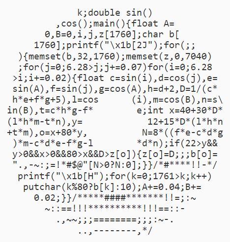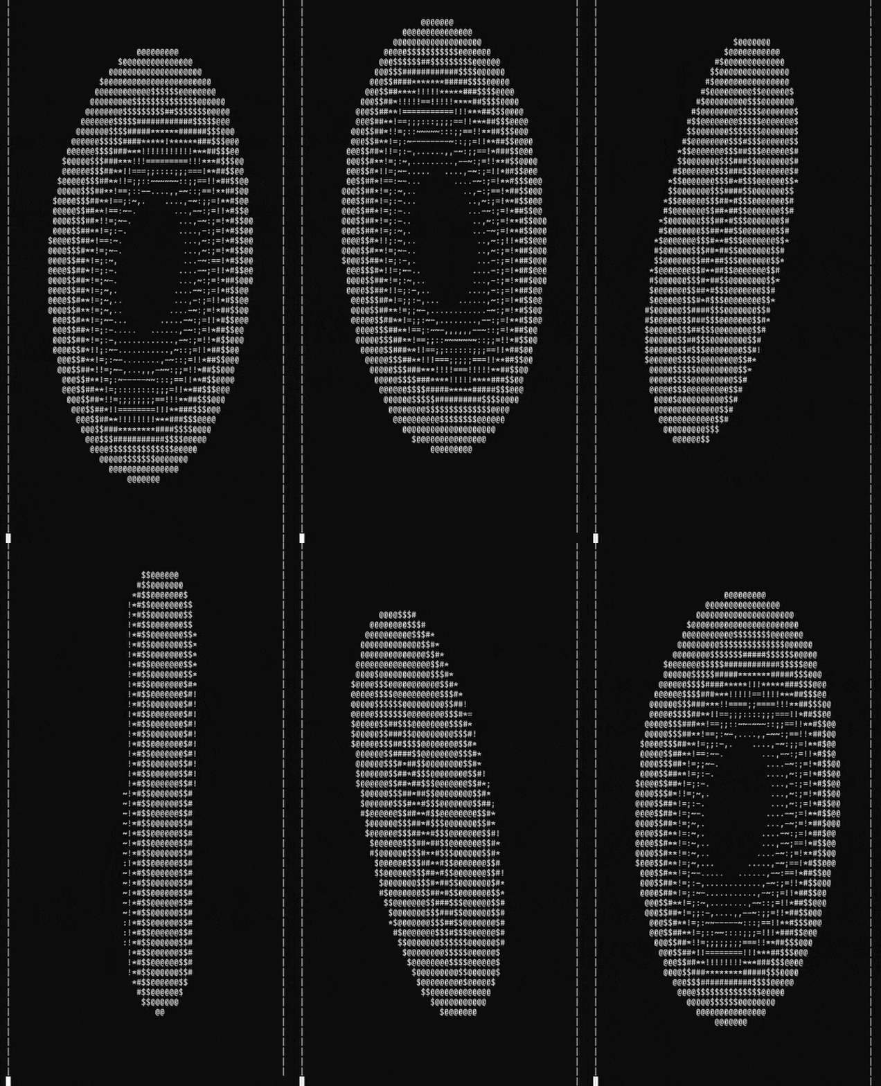
The Donut Code spinning Donut.

There has been an image in my mind for several years since I first saw it. "Donut-shaped C code that generates a 3D spinning donut" was, if I'm not mistaken, the video where I first saw it. For a long time this piece of code seemed magical to me. Even after unpacking it I was uncapable of decyphering that chaotic mess of variables lacking semantic meaning. I never gave it the importance nor the attention it deserved, as I thought of it as no more than intellectual foreplay among programmers.

However, some days ago I became obsessed with the topic and, after some afternoons filled with linear algebra and Python, I discovered that it was in fact something quite simple. My objective wasn't to arrive at something even remotely close to that code, but rather to experiment with the math involved from the ground up. I've been careful not to read absolutely anything about how lightning, projections or whatever works. As one would expect, the results haven't been perfect, but it was an interesting experience.

1. The Objective

The final goal is simple: to show a 3D donut dancing on screen. Attacking this problem from the perspective of algorithms tends to yield inefficient or spaghetti code, so let's forget that computers exist for a while and work with pure math. We can subdivide the problem into five more simple ones:

Describe all of the donut's (or torus ) points using parametric equations.
Make the donut "dance" using matrices.
Give each point of the donut a brightness value.
Project the donut's points on a 2D plane.
Go from the plane to the terminal and show the donut on screen.

After solving all of that, we will write the corresponding code in Python and transfer it to C, where we will reduce it to its minimum expression and give it the shape of a donut.

2. The Donut

The parametric equations describing a torus centered along the z axis are the following:

\[x = \cos(u) (R + r \cos(v))\] \[y = \sin(u) (R + r \cos(v))\] \[z = r \sin(v)\]

(In the beginning I looked up these equations, but after a while I realized that they are the result of applying a rotation matrix on a circunference shifted from the origin. It's not really important, but I think it's cool)

(Figure 2) u and v describing points on the torus. — (Figure 2) \(u\) and \(v\) describing points on the torus.

Transferring this to code is trivial. Inside the class Torus we have the following method:

class Torus

				def point_at(self, u, v):
    x = np.cos(u) * (self.R + self.r * np.cos(v))
    y = np.sin(u) * (self.R + self.r * np.cos(v))
    z = self.r * np.sin(v)

    return np.array([x, y, z])

It could seem arbitrary to center it on the z axis, however we are going to spin everything when we apply the rotation matrices, so it won't be important.

3. The Dance

Given any of the donut's points, we can apply linear transformations to it through matrices. We don't need anything fancy, so some simple rotations should do the trick. The angle \(\theta\) will vary to convey movement.

\[ \begin{pmatrix} 1 & 0 & 0 \\ 0 & \cos(\theta) & -\sin(\theta) \\ 0 & \sin(\theta) & \cos(\theta) \end{pmatrix} \]

We can also move the donut up and down very slightly:

\[y(\theta) = \cos(\theta)\]

4. The Light

Determining a point's brightness would be extremely simple if only shadows didn't exist. As it was my intention to finish this quick and without any external resource, we will simply ignore this problem.

Basically, if a beam of light hits a surface perpendicularly, the point where it lands will reach its maximum brightness. The greater the angle, the darker the surface.

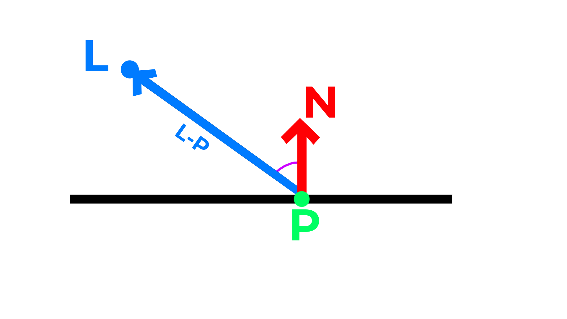
We can ask the same question by looking at how aligned is the normal to the surface to the vector that goes from the light source to the surface (bit of a mouthful, I know). (Figure 3)

(Figure 3) The smaller the angle formed between N and L-P, the bigger the brightness at that point. — (Figure 3) The smaller the angle formed between \(N\) and \(L-P\) , the bigger the brightness at that point.

The operation to find out how aligned are two vectors is the scalar product, and to only get values from 0 to 1 (included) we have to previously normalize both vectors.

\[\vec{V} = L - P\] \[\vec{v} = \frac{\vec{V}}{\mid \vec{V} \mid}\] \[\textrm{brightness} = \vec{v} \cdot \vec{N}\]

Now we only have to get the normal to the surface of the torus on a given point. If we imagine taking a small step along \(u\) (in other words, \(\textrm{torus}(u + du, v)\) ), we'll end up on a new point. It's worth noting that if we take the same step along \(v\) (in other words, \(\textrm{torus}(u, v + dv)\) ), we'll have moved perpendicularly to the previous direction. This is useful, as we can define the plane tangent to the torus' surface at that point using both vectors. Getting the normal to that plane is easy.

Before doing that though, let's formalize what we mean when saying "a small step". What we are really doing is calculate the derivatives to the parametric equations with respect to \(u\) and \(v\) in all coordinates, that is:

\[\frac{dx}{du} = \frac{d}{du}(\cos(u)(R + r\cos(v))\] \[\frac{dy}{du} = \frac{d}{du}(\sin(u)(R + r\cos(v)))\] \[\frac{dz}{du} = \frac{d}{du}(r\sin(v))\] \[\\\] \[\frac{dx}{dv} = \frac{d}{dv}(\cos(u)(R + r\cos(v))\] \[\frac{dy}{dv} = \frac{d}{dv}(\sin(u)(R + r\cos(v)))\] \[\frac{dz}{dv} = \frac{d}{dv}(r\sin(v))\]

We can form two vectors out of this set of equations, let's call them \(\frac{d\vec{V}}{du}\) and \(\frac{d\vec{V}}{dv}\) . As we've said, these vectors are ortogonal and lie on the plane tangent to the torus' surface at that point, so their cross product will yield another vector normal to that surface.

How do we decide the order of the terms in this product? We could reason through it, but really it's a 50/50 chance, so we can pick at random and see how it looks, in this case:

\[\vec{N} = \frac{d\vec{V}}{dv} \times \frac{d\vec{V}}{du}\]

The resulting function which also normalizes all vectors is:

class Torus

				def normal_at(self, u, v):
    dV_du = np.array([-np.sin(u)*(torus.R + torus.r * np.cos(v)),
                        np.cos(u)*(torus.R + torus.r * np.cos(v)),
                        0])
    dV_dv = np.array([-torus.r*np.cos(u)*np.sin(v),
                        -torus.r*np.sin(u)*np.sin(v),
                        torus.r*np.cos(v)])
    normal = np.cross(dV_dv, dV_du)
    normal = normal / np.linalg.norm(normal)
    return normal

When doing the scalar product \(\vec{v} \cdot \vec{N}\) , we can get negative values, which simbolize that the surface is "giving its back" to the light source, hence we can interpret those as zero. Again, the resulting function is:

Brightness

				def brightness_at(torus, u, v, rotation_matrix, light_source):
    point = rotation_matrix @ torus.point_at(u, v)
    normal = rotation_matrix @ torus.normal_at(u, v)
    d = light_source - point
    d = d / np.linalg.norm(d)

    brightness = np.dot(d, normal)

    if brightness < 0:
        return 0
    else:
        return brightness

5. The Projection

Given a plane and a point outside that plane, the projection of that point on the plane will be the point moved along a line perpendicular to the plane until reaching it. To find out the distance from the point to the plane we can create a vector \(\vec{v}\) that goes from the origin of the plane to the desired point and take its scalar product with the normal of the plane. The projection will consist on subtracting the normal to the plane scaled by the distance to the point. This achieves a perpendicular movement that ends up with the point lying at the plane.

class Plane

				def project(self, point):
    v = point - self.Origin
    distance = v.dot(self.Normal)
    projected_point = point - distance * self.Normal

    return projected_point

(This is NOT the standard way of projecting to a screen. Then again, I was doing this as intelectul foreplay and not as something professional)

6. The Terminal

Let's first establish the origin of the plane as our frame of reference.

class Plane

				def relative_coords(self, point):
    return point - self.Origin

Our frame of reference is now centered at the plane's origin. However the origin of the terminal is located at its top-left corner, and its coordinates increase from left to right and from top to bottom. If we know how many rows and columns our terminal has (which we know because we have predetermined it), this isn't a problem:

Terminal Coordinates

				def plane_coords_to_terminal_coords(plane_coords):
    col = int(COLS/2 + plane_coords[0])
    row = int(ROWS/2 - plane_coords[2])

    return (row, col)

# main
projected_point = plane.project(torus_point)
projected_point = plane.relative_coords(projected_point)
(row, col) = plane_coords_to_terminal_coords(projected_point)

What follows is obvious. We take that brightness value and we assign a character to a list that represents each coordinate in the terminal.

def main()

				brightness = brightness_at(torus, u, v, rotation_matrix, light_source)
character = brightness_to_character(brightness)
screen[row][col] = character

The function association a character to each brightness value can be freely chosen, but I will stick to the original set of characters.

Bright2Char

				def brightness_to_character(brightness):
    # brightness -> [0..1]
    # characters -> [0..11]
    index = round(brightness*11)
    characters = ".,-~:;=!*#$@"
    return characters[index]

Actually there's a last thing to consider. Different point on the donut with different brightness values can project to the same spot on the terminal, meaning the output on the terminal will pick the latest projected value and not the one that makes sense tridimensionally.

As I said at the beginning of this article, we won't focus on perfectioning this, although picking the value with the highest brightness found yields a pretty decent result.

Result

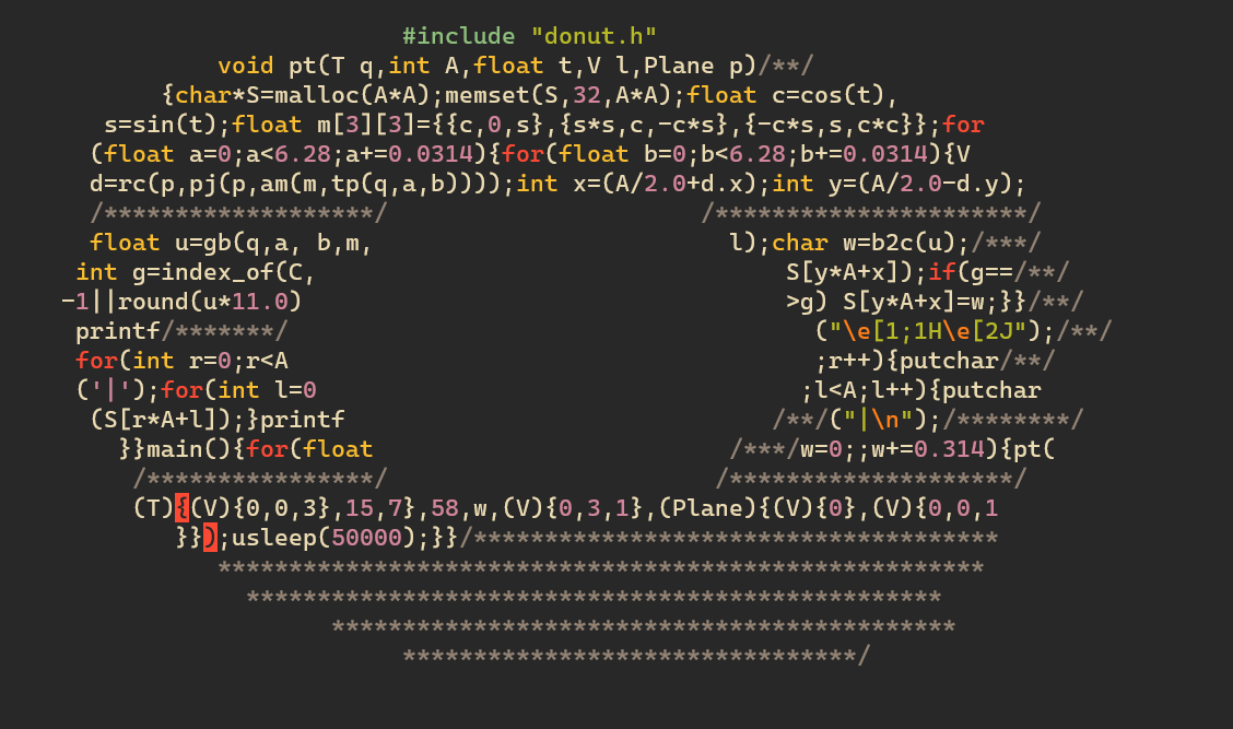
That's it! The full code is available at my GitHub . It's not the best, but that's what you get for improvising. When transformed to C and reduced as much as possible, it can be massaged into a donut shape.

Going from Python to C is not difficult but rather tedious, as we can't use NumPy, but it's doable. The translated code is also available on my GitHub. It's amazing how quick it is in comparison.

However this code is too long to be shaped like a donut (or at least to an aesthetically pleasing one), so we must simplify it further. This is when I cheated a little, as I didn't only cram together everything I could, but I also put a lot of functions in the file donut . I don't think this is too bad, as we could have used an external linear algebra library in the first place.

With this smaller code we only have to eliminate unnecesary spacing and give the code the desired shape. I did this by eye (you don't have to use fancy techniques for everything). To fill in the gaps I used some comments, et voilá .

26/02/2024